A* pathfinding algorithm
Game development introduced me to programming when I was around 10 years old, and I’ve loved it ever since. One of the first formal algorithms I learned before entering university was A* (pronounced “A star”), and I really had a great time learning about it. It’s one of the most widely used pathfinding algorithms and is one that you would likely be introduced to first when approaching the subject of pathfinding. A pathfinding algorithm takes a start point (also known as a node) and a goal and attempts to make the shortest path between the two given possible obstacles blocking the way.

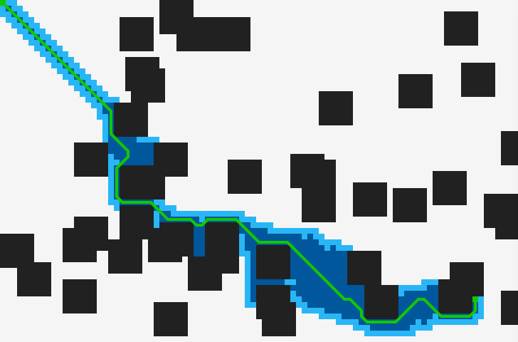
I’ve always thought the simplest example of pathfinding is a 2D grid in a game, it can be used to find a path from A to B on any type of graph. For example a graph where vertices are airports and edges are flights, A* could be used to get the shortest trip between one airport and another.
I’ve always thought the simplest example of pathfinding is a 2D grid in a game, but it can be used to find a path from A to B on any type of graph. For example a graph where vertices are airports and edges are flights, A* could be used to get the shortest trip between one airport and another.

Properties
A* has the following properties:
- It is complete; it will always find a solution if it exists.
- It can use a heuristic to significantly speed up the process.
- It can have variable node to node movement costs. This enables things like certain nodes or paths being more difficult to traverse, for example an adventurer in a game moves slower across rocky terrain or an airplane takes longer going from one destination to another.
- It can search in many different directions if desired.
How it works
It works by maintaining two lists; the open list and the closed list. The open list’s purpose is to hold potential best path nodes that have not yet been considered, starting with the start node. If the open list becomes empty then there is no possible path. The closed list starts out empty and contains all nodes that have already been considered/visited.
The core loop of the algorithm selects the node from the open list with the lowest estimated cost to reach the goal. If the selected node is not the goal it puts all valid neighboring nodes into the open list and repeats the process.
Part of the magic in the algorithm is that all created nodes keep a reference to their parent. This means that it’s possible to backtrack back to the start node from any node created by the algorithm.
Node
A node has a positioning value (eg. x, y), a reference to its parent and three ‘scores’ associated with it. These scores are how A* determines which nodes to consider first.
G score
The g score is the base score of the node and is simply the incremental cost of moving from the start node to this node.
H score - the heuristic
The heuristic is a computationally easy estimate of the distance between each node and the goal. This being computationally easy is very important as the H score will be calculated at least once for every node considered before reaching the goal. The implementation of the H score can vary depending on the properties of the graph being searched, here are the most common heuristics.
Manhattan distance
This is the simplest heuristic and is ideal for grids that allow 4-way movement (up, down, left, right).

Diagonal distance (uniform cost)
This heuristic is used for 8-way movement (diagonals) when the cost of diagonal movement is the same as the cost of non-diagonal. Note that this is very inaccurate if the costs for diagonal and non-diagonal are not the same.

Diagonal distance
This heuristic is used for 8-way movement when the cost of diagonal movement differs from the non-diagonal cost. Remember that the cost of diagonal distance doesn’t need to be exact and is usually worth it to use a constant multiplier rather than the square root as the square root operation is quite expensive.

Euclidean distance
This heuristic can be used when movement is possible at any angle, it can also be quite expensive and may be worth considering a less expensive function.
You should avoid using the square root all together and calculate h(n)^2. Then make sure that g(n)^2 is used to ensure both are relative.

F score
The f score is simply the addition of g and h scores and represents the total cost of the path via the current node.
Pseudocode
This pseudocode allows for 8-way directional movement.
function A*(start, goal)
  open_list = set containing start
  closed_list = empty set
  start.g = 0
  start.f = start.g + heuristic(start, goal)
  while open_list is not empty
    current = open_list element with lowest f cost
    if current = goal
      return construct_path(goal) // path found
    remove current from open_list
    add current to closed_list
    for each neighbor in neighbors(current)
      if neighbor not in closed_list
        neighbor.f = neighbor.g + heuristic(neighbor, goal)
        if neighbor is not in open_list
          add neighbor to open_list
        else
          openneighbor = neighbor in open_list
          if neighbor.g < openneighbor.g
            openneighbor.g = neighbor.g
            openneighbor.parent = neighbor.parent
  return false // no path exists

function neighbors(node)
  neighbors = set of valid neighbors to node // check for obstacles here
  for each neighbor in neighbors
    if neighbor is diagonal
      neighbor.g = node.g + diagonal_cost // eg. 1.414 (pythagoras)
    else
      neighbor.g = node.g + normal_cost // eg. 1
    neighbor.parent = node
  return neighbors

function construct_path(node)
  path = set containing node
  while node.parent exists
    node = node.parent
    add node to path
  return path
Optimisation
The primary opportunity for optimisation is in selecting the right data structure for the open list. While it’s possible to implement the open list with any list data structure, the best choice is a list that has both a fast insert and extract minimum operation. The performance of the insert operation is more important than extract minimum since the algorithm typically doesn’t extract all nodes inserted into the open list, with the exception being when no path exists).
These properties are typical of priority queues, such as a binary heap which features an Θ(\log n) time complexity for both its insert and extract minimum operations. The Fibonacci heap can optimise this even further with its Θ(1) insert and O(\log n) extract minimum.
Another less frequent operation that occurs is decrease key, when the g cost of a node in the open list needs updating. The Fibonacci heap again comes out on top in this regard with a Θ(1) decrease key time complexity.
| Data structure | Insert | Extract minimum | Decrease key |
|---|---|---|---|
| Array | Θ(1)* | O(n) | Θ(1) |
| Sorted array | O(\log n) | Θ(1) | O(n) |
| Binary heap | Θ(\log n) | Θ(\log n) | Θ(\log n) |
| Fibonacci heap | Θ(1) | O(\log n)* | Θ(1)* |
* Amortised
Demo
See the algorithm in action along with Dijkstra’s algorithm in the pathfinding visualiser web app I created. The source is available on GitHub.
Textbooks
Here are two CS textbooks I personally recommend; the Algorithm Design Manual (Steven S. Skiena) is a fantastic introduction to data structures and algorithms without getting to deep into the maths side of things, and Introduction to Algorithms (CLRS) which provides a much deeper, math heavy look.


